3. Automatic Input Selection
General Idea of Input Selection
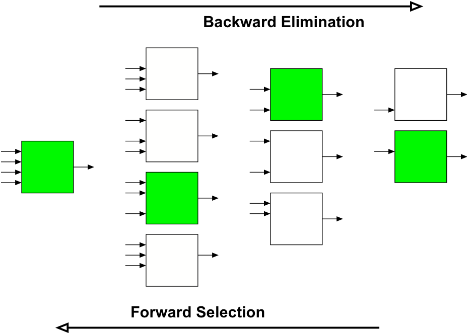
- Forward Selection (FS)
- fast
- recommended for many potential inputs but only few selected
- ignores correlations/interactions between potential inputs - Backward Elimination (BE)
- slower
- recommended if most potential inputs are selected
- takes into account correlations/interactions between potential inputs - Stagewise Selection
- combination of FS and BE - Brute Force
- all input combinations
Input Selection - What for?
Input Selection in the Context of Machine Learning
For choice of optimal model complexity, input selection evaluates merits of input subsets
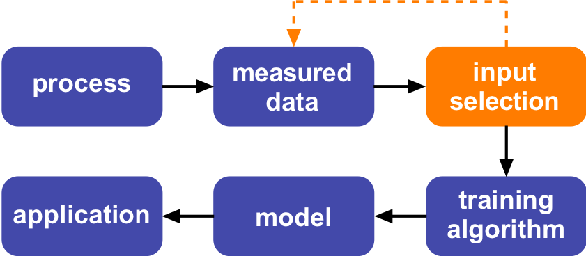
Motivation
- Optimal bias/variance trade-off
- Explore relevance of inputs
Aims
- Weakening the curse of dimensionality
- Reducing the model’s variance error
- Increase of process understanding
- More concise and transparent models
- May support future design of experiments (DoE) or active learning strategies

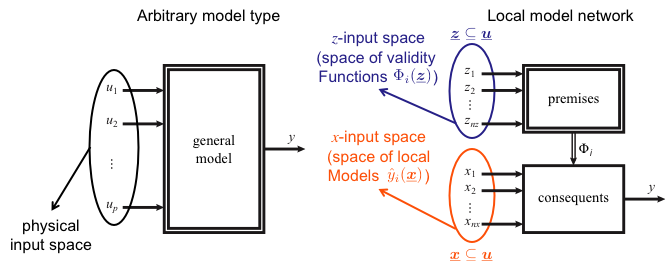
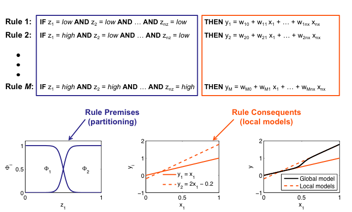
Local Model Networks Enhanced
Separate Inputs for Local Models and Validity Functions
- Whole problem split into smaller sub-problems
- Training algorithm necessary
- Here: Hierarchical Local Model Tree (HILOMOT)
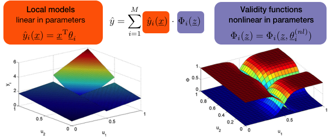
Separation between Linear and Nonlinear Effects
- LMNs Reveal Possibility to Separate between Linear and Nonlinear Effects
- Any physical input ui can be included in the rule premises zi and/or in the rule consequents xi
- The separation between linear and nonlinear effects is not possible for other types of models
- In the following the rule premises are referred to as the z-input space, the rule consequents are referred to as the x-input space
Equivalence to Fuzzy
Interpretation as Takagi-Sugeno Fuzzy System
Input Selection With the HILOMOT-Algorithm
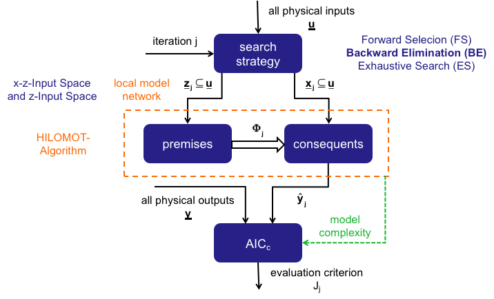
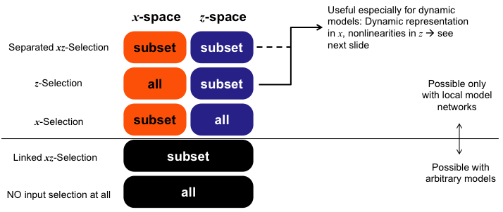
Input Spaces
Overview: Different Selection Strategies for Input Selection Tasks
Depending on the selection strategy either subsets or all physical inputs can be assigned to the x- and z-input space.
Demonstration Example: HILOMOT Wrapper Method
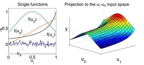
Artificial Process
- Superposition of:
- Hyperbola f(u1)
- Gaussian function f(u2)
- Linear function f(u3)
- Normal distributed noise, σ = 0, σ = 0.05 (for u4)

Setting
- Training samples N = 625 & N = 1296
- Placed on a 4-dimensional grid
HILOMOT Wrapper Settings
- Evaluation criterion: Akaike’s information criterion (AICc)
- Search Strategy: Backward elimination (BE)
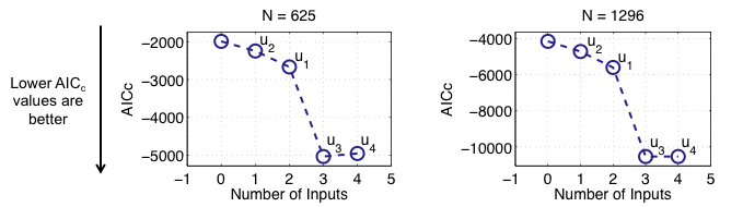
4-D Demonstration Example: Linked x-z-Selection
Results for the Linked x-z-Selection
- Because of the BE search strategy, the results have to be read from right to left
- Each ‘o’ is labeled with the input that is discarded in the corresponding BE step
- A growing sample size N reduces the bad influence of the useless input u4
- For both sample sizes N, the HILOMOT wrapper method identifies the 4th input as not useful in the linked x-z-space
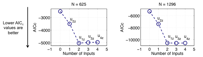
4-D Demonstration Example: z-Selection
Results for the z-Selection
- Inputs u3 and u4 are identified as useless in the z-space
- Because the slope in u3 direction does not change, no partitioning has to be done in that direction - As soon as an important input in the z-space is removed the evaluation criterion gets significantly worse
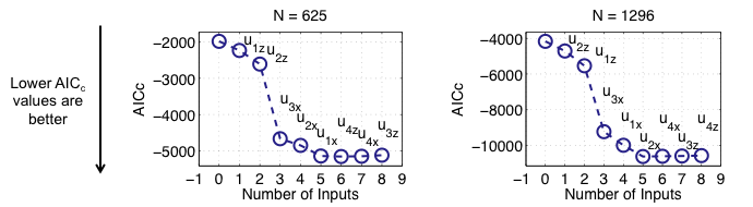
4-D Demonstration Example: Separated x-z-Selection
Results for the Separated x-z-Selection
- Input u4 is identified as useless in the x- as well as in the z-space for both sample sizes N
- Input u3 is identified as useless in the z-space for both sample sizes N
- After the first useful input is discarded, the evaluation criterion gets slightly worse
Real-World Demonstration Examples

Auto Miles Per Gallon (MPG) Data Set
(From the UCI Machine Learning Repository (http://archive.ics.uci.edu/ml) 2010)
- N = 392 samples
- q = 1 physical output:
- Auto miles per gallon - p = 7 physical inputs:
- Cylinders (u1)
- Displacement (u2)
- Horsepower (u3)
- Weight (u4)
- Acceleration (u5)
- Model year (u6)
- Country of origin (u7) - Data Splitting
- ¾ of data: training samples (used for network training, complexity selection, input selection)
- ¼ of data: test samples (only for final testing)
- Heuristic, deterministic data splitting strategy
Auto MPG Wrapper Input Selection Results
Results for the x-z-Input Selection
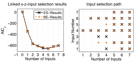
- Both search strategies yield similar results:
- Best AICc-Value for 5 inputs
- Same input combination - Input selection path:
- Indicates the input combination to a given number of inputs
- In case of BE read from right to left
Results on the Test Data
- Mean squared error (MSE) for best AICc-Values:
- MSE (5 inputs) = 6.0
- MSE (all inputs) = 7.7 - Most important inputs: u4 (car weight) and u6 (model year)
- Improvement of model accuracy
- Information about very important inputs
Results for the z-Input Selection
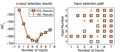
- Best AICc-Value ES result:
- 4 inputs - Best AICc-Value BE result:
- 4 inputs
- BUT other input combination(see input selection path)
Results on the Test Data
- MSE for best AICc-Values:
- MSE (best ES) = 5.2
- MSE (best BE) = 5.3
- MSE (all inputs) = 7.7 - Most important inputs: u2 (displacement) and u6 (model year)
- Improvement of model accuracy
- Information about nonlinear input influences
Climate Control
Process
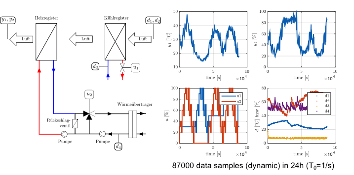
- 2 controlled inputs (u1, u2)
- valve positions - 4 measured inputs (d1, d2, d3, d4)
- temperature, rel. humidity, temp., temp. - 2 measured outputs (y1, y2):
- temperature, rel. humidity - Difficult modeling with ARX: Unstable models are possible
Selection
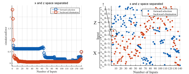
- Selection on the simulated output of validation data.
- Backward selection gives significantly better results.
- ~15 inputs/regressors are sufficient for a good model.
- Allowed delays: (k-1) … (k-10).
- Forward selection: Tries to model the process with multiple nonlinear influences.
- Backward selection: Nonlinearities only need to be considered in u1(k-1) and u2(k-2)!
Next Chapter: 4. Metamodeling Back to Overview