5. Nonlinear Dynamic Models (Local Model Networks with OBF and FIR)
Dynamic Representations
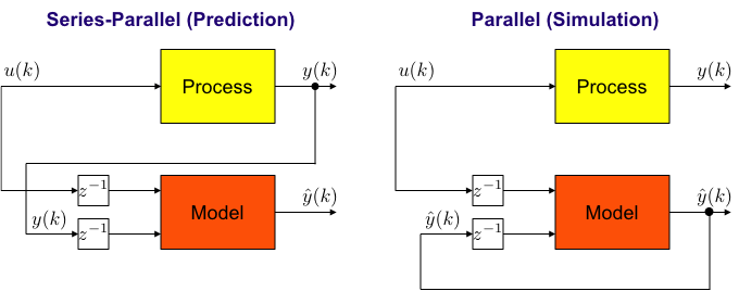
Disadvantages of Traditional Nonlinear Dynamic Models
- One-step-ahead prediction error (series-parallel configuration) is optimized (usually).
- Tuning in simulation (parallel configuration) possible → Complex nonlinear problem.
- Simulation can even become unstable → Unreliable.
- Online adaptation thus is very risky.
NARX
- Problems with stability due to external output feedback.
- Very sensitive w.r.t. correct order and dead time.
- Interpolation → Strange effects.
- Optimization of equation error (in series-parallel). Drawbacks:
- emphasis on high frequencies
- one common denominator A(z) → identical dynamics for all inputs
NFIR
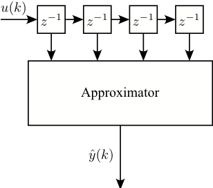
- No problems with stability because no feedback.
- Optimization of simulation error → All NARX difficulties are gone.
- New Drawback: Huge orders/dimensions necessary.
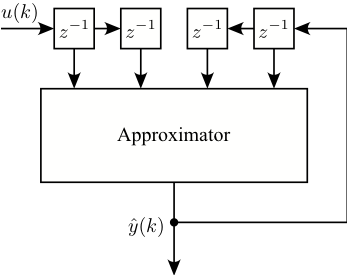
NOBF
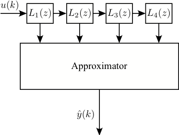
- No problems with stability because only local feedback.
- Optimization of simulation error → All NARX difficulties are gone.
- New Drawback: Selection of filter pole(s)?
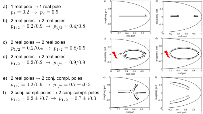
What's Bad With NARX? Interpolation of 2 ARX Models
What's Bad With NARX? Extrapolation

- Extrapolation behavior in the y(k‒i)-axes determines dynamics
- slope ≈ 0 → static
- |slope| < 1 → stable dynamics
- |slope| > 1 → unstable dynamics - Big advantage for all linearly extrapolating model architectures like local linear ...
- Extremely dangerous for polynomials.
- Most other model architectures extrapolate constantly.
What's Bad With NARX? MISO Models
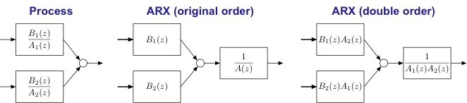
- Each input → output: Individual dynamics.
- One common denominator A(z).
- Multivariate ARX model requires high order = sum of individual orders.
- Approximate zero/pole cancellations.
- Static inputs: Bi (z) needs to cancel A(z).
- Popular solution in linear case → Subspace identification in state space(FIR-based approach)
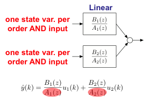
But Even With NOE? MISO Models
- OE: Linear case, each input:
- individual transfer function
- individual feedbacks
- individual states
- no. of state variables = no. of inputs x order
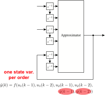
- NOE: Nonlinear case, each input:
- one feedback independent of inputs
- one set of states
- no. of state variables = order
Regularized FIR Estimation – The Linear Case
Recent Progress for the FIR Identification Case
- Usage of regularization for the estimation of linear FIR models (proposed by Pillonetto et. al. 2011)
Modified Loss Function for FIR Estimation
- Regularized least squares problem
- Choice of the regularization matrix
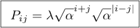
- “Tuned correlated” (TC) kernel, penalizes an exponentially decaying version of the first order derivative of the system
- Interpretation as RKHS or Gaussian Process Model
- Nonlinear optimization of the hyperparameters
Regularized FIR
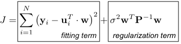
- Loss function

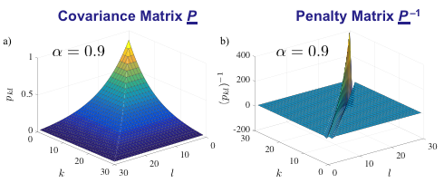
- P specifies the parameter covariances
- P should decrease exponentially with α (α is the pole)

- P also should decrease exponentially with distances k-l.

This is the TC kernel: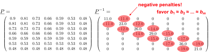
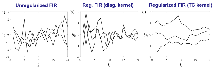
3 Priors ~ Gaussian Process  3 Realizations each, order m = 20
with: 
b) white, bk independent, exp. decreasing
c) correlated, bk dependent, exp. decreasing
Example: Identification of Damped Second Order System
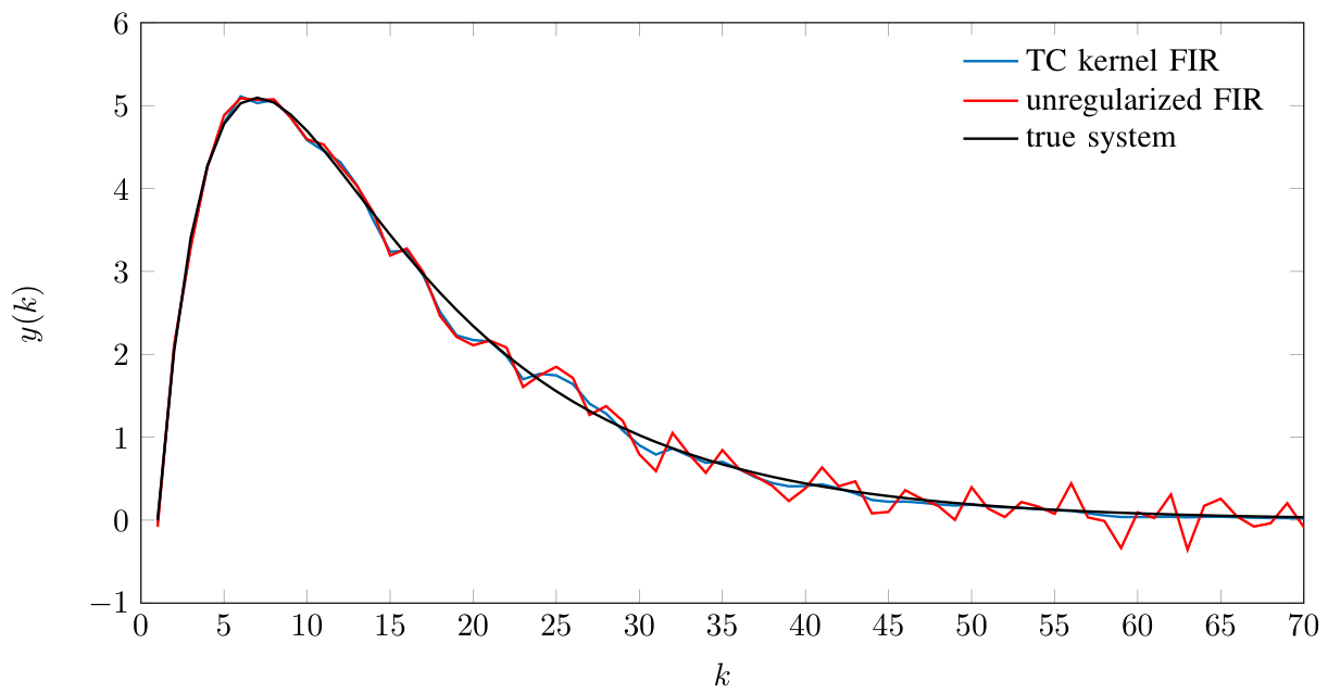
Advantages of Regularized FIR (Blue Curve)
- High variance of FIR is suppressed
- Compared to ARX the stability of the impulse response is a priori guaranteed
Extension to the Nonlinear Case – Concept
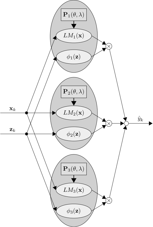
Idea
- Use regularized FIR models as local Models
- Validity functions z can depend on delayed inputs and outputs either
Advantages
- Complete model trained for simulation error
- Stability of the identified model is guaranteed
- Model order estimation is not required
Disadvantage
- Hyperparameter search for every local model
Further aspects
- Consideration of the LMN offset in the models
- Interpretation of model error as a composition of nonlinearity and noise error
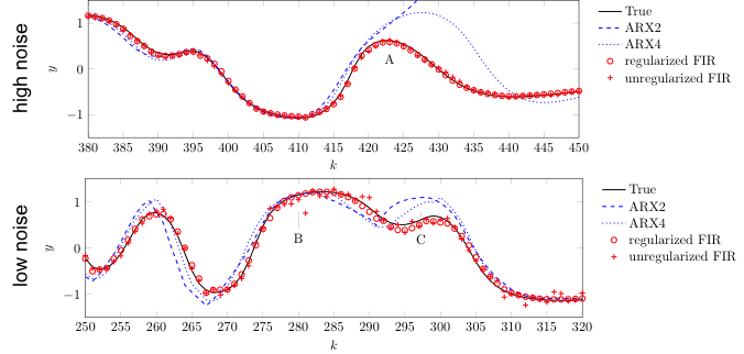
Example: Saturation Type Wiener System
![]()
Estimated Results with LOLIMOT and Different Local Model Types
Next Chapter: 6. Classification Back to Overview