Research Topics Christopher Illg
Nonlinear Regularized FIR Models
System identification concerns the estimation of dynamic models from finite, noisy measurement data. Additionally, some prior knowledge can be incorporated with simple structural assumptions. This procedure is called gray-box modeling.
The idea proposed in [6] corresponds to a gray-box modeling approach for estimating finite impulse response (FIR) model structures. FIR models have no output feedback, whereas the external feedback makes ARX models so powerful. However, this comes with some drawbacks for the ARX models: biased parameter estimation, equation error configuration, and problems with multivariate feedback [2]. On the other hand, the parameter estimation of FIR models is unbiased, they are in the output error configuration and are inherently stable. Usually, the estimation of FIR models requires a high number of parameters, which leads to a high variance error. Regularization can be used to overcome this problem. Prior knowledge can be incorporated by introducing an additional penalty term in the estimation procedure. This regularization term introduces a relationship between the parameters of the FIR model themselves.
To apply the regularized FIR models easily in the nonlinear domain, local model networks (LMNs) can be used. The output of an LMN is calculated as an interpolation of local models (LMs) with the associated validity functions Φi, i = 1, ..., M [5]. The input of the LMs is spanned by x(k), while the input of the validity functions allows for a different space z(k) (see Figure 1) [3]. The validity functions can be determined by incremental tree-based construction algorithms with axis-orthogonal or axis-oblique partitioning [5].
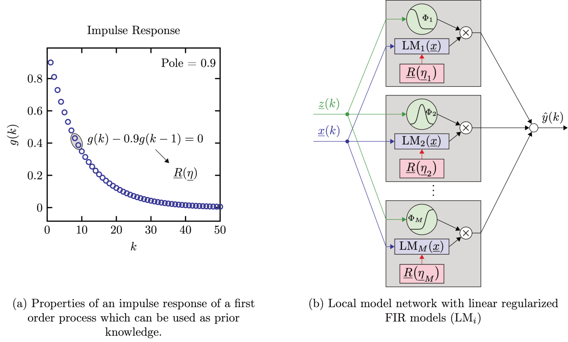 |
| Figure 1: Nonlinear regularized FIR models |
Nonlinear Laguerre and Kautz Models
Nonlinear dynamic models are the basis for most sophisticated methods in e.g., prediction, simulation, optimization, control, fault detection, and diagnosis. The most popular approach in nonlinear system identification is establishing a regressor space with filtered inputs and optionally filtered outputs gathered in the regressor vector x. The nonlinear system behavior itself is then modeled by a universal approximator (NL), see Figure 2.
The choice of the regressor vector x is crucial for modeling the dynamics. On the one hand, the vector can consist of (a) only delayed versions of the input (FIR) or internal filtering of the input by using cascades of filters with (b) a real pole (Laguerre) or (c) a complex pole pair (Kautz) [1]. Laguerre and Kautz input spaces allow for a significantly reduced dimensionality of the regressor space compared to the FIR regressor space since lower model orders can capture the significant process dynamics. The pole(s) p is a hyperparameter and can be optimized or chosen heuristically. On the other hand, also (d) a combination of delayed versions of the input and output (ARX) is possible where external feedback is used.
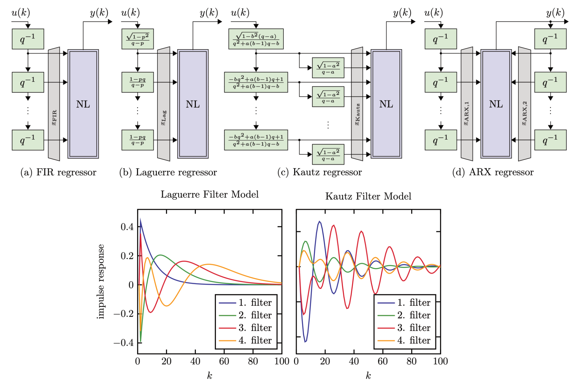 |
| Figure 2: Different regressor spaces which depend only on filtered/delayed versions of the input (FIR, Laguerre, Kautz) and one using external feedback (ARX) with xARX = [xARX,1,xARX,2]. The NL block represents the universal approximator, which models the static nonlinearity. |
Model Predictive Control with Local Model Networks
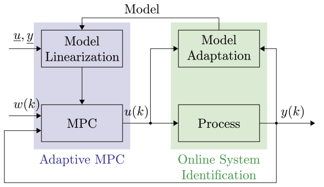
The main task in model predictive control (MPC) is to predict the future output of the process and estimate an optimal sequence for the manipulated variable with respect to an objective function. To control nonlinear processes with an MPC, oftentimes, the nonlinear process model is first linearized, and the linearized model is used to predict the next time steps. The advantage of a linear model in the MPC is given by a closed-form solution, which is computationally efficient and yields a global optimum.
For the internal model, a local model network (LMN) with regularized finite impulse response (FIR) models can be chosen. The linear model in the current operating point can easily be calculated by interpolating the model parameters of all local models. Regularized FIR models are well-suited for online identification as they are inherently stable. Further advantages are e.g. the linearity in the parameters, the output error configuration, and the insensitivity w.r.t. a wrong model order or wrong dead times. Additionally, regularization improves the robustness of the closed-loop online identification procedure [4]. For the online system identification of the local models of the LMN, a recursive weighted least squares (RWLS) method can be applied. A block-diagram of an adaptive MPC in shown in Figure 3.
|
| Figure 3: Adaptive model predicitve control with online system identification. |
References
| [1] | Paul M.J. Van den Hof, Peter S. C. Heuberger, and J. Bokor. “System Identification with Generalized Orthonormal Basis Functions”. In: Proceedings of 1994 33rd IEEE Conference on Decision and Control. IEEE, 1994. |
| [2] | Christopher Illg, Tarek Kösters, and Oliver Nelles. “Handling of Time Delays in MISO Processes with Reg- ularized Finite Impulse Response Models”. In: 2024 European Control Conference (ECC). 2024, pp. 3545– 3550. |
| [3] | Christopher Illg, Tarek Kösters, and Oliver Nelles. “On the Choice of the Scheduling Variables for Dynamic Local Model Networks with Local Regularized FIR Models”. In: 2024 IEEE International Conference on Fuzzy Systems (FUZZ-IEEE). 2024, pp. 1–8. |
| [4] |
Christopher Illg and Oliver Nelles. “Adaptive Model Predictive Control with Regularized Finite Impulse Response Models”. In: ATHENA Research Book, Volume 1 1 (2022), pp. 327–331. |
| [5] | Oliver Nelles. Nonlinear System Identification from Classical Approaches to Neural Networks, Fuzzy Systems, and Gaussian Processes. 2nd ed. Springer International Publishing AG, 2021. |
| [6] | Gianluigi Pillonetto and Giuseppe De Nicolao. “A New Kernel-based Approach for Linear System Identification”. In: Automatica 46.1 (Jan. 2010), pp. 81–93. |