Research Topics Geritt Kampmann

Back to Overview

 

Robust One- and Two-Class Classifiers via Zero Leave-One-Out Cross-Validation Errors

One-class classifiers [1, 2] are often used to detect changes in data over time (novelty detection). If the data is collected online through sensors on a technical system, these changes may be caused by environmental changes (e.g. temperature) or by changes of the system itself that indicate the need for maintenance or even an imminent malfunction.

Another application of one-class classifiers might be the detection of extrapolation when using models generated from data. If a model output is calculated for input data that lies far away from the data used for training, a rather large model error should be expected. The results should only be used very carefully depending on the application.

For this kind of applications, the use of Radial Basis Function (RBF) Networks is proposed [3]. In the simplest case one Gaussian function is placed on every data point and the classifier is a weighted sum of all Gaussians. The weights (parameters) can be calculated efficiently using regularized least-squares (ridge regression). Regularization is necessary because the number of parameters equals the number of data points, which causes overfitting of the data and numerical problems if data points are (almost) identical.

Now the problem occurs, that before the weights of the RBF Network can be calculated two hyperparameters have to be determined:

• the standard deviation of the Gaussians σ, and
• the regularization strength λ.

The influence of the regularization strength can be observed in Fig. 1. With increasing λ the weights are decreased, resulting in a more robust estimation, but also leading to closer boundaries and, when overdone, to misclassifications (Fig.1 bottom right).

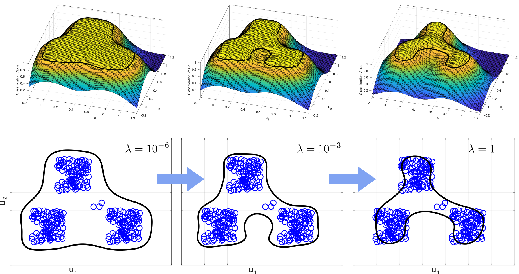Figure 1: Influence of the regularization strength λ on the classification boundary.

 

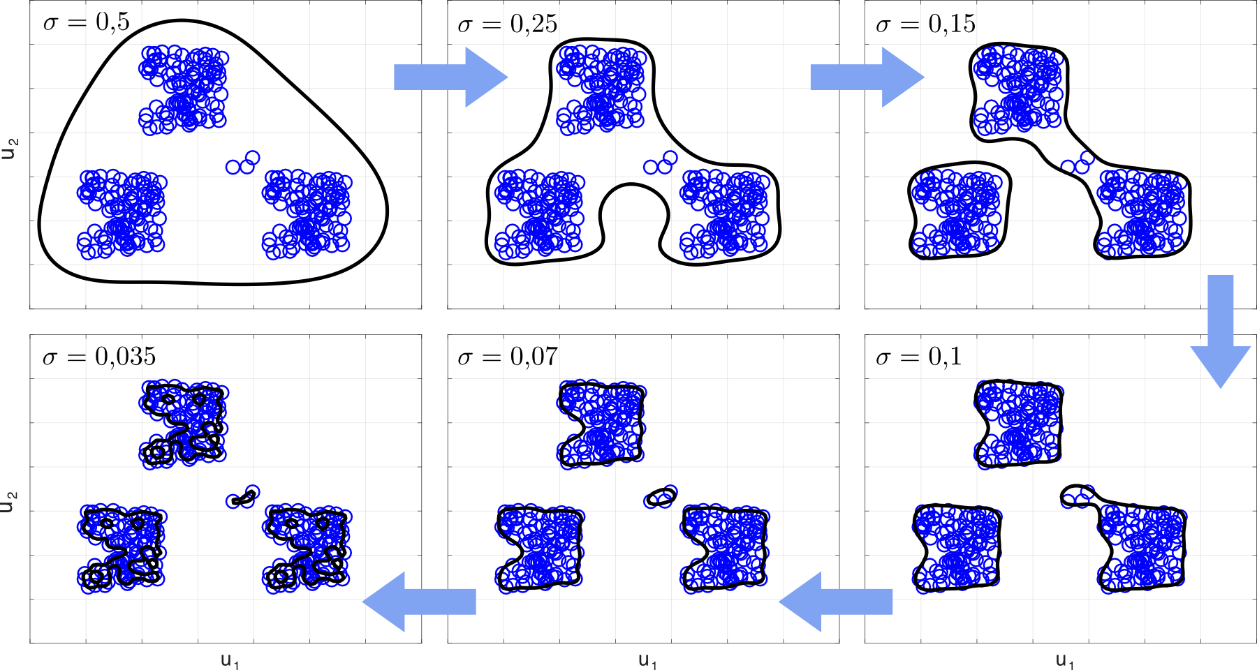
The influence of the standard deviation is depicted in Fig. 2. From top left to bottom right σ is reduced, causing the boundary to move closer to the data. Depending on σ, the data is separated in one, two, three and even four groups, before (in the bottom, left diagram) the data finally is starting to be dissolved in an unwanted number of random pieces.

Figure 2: Influence of the standard deviation σ on the classification boundary.

 

The question remains, how to select the hyperparameters in a useful fashion. From the range of the data, the number of the data points and the number of dimensions the useful range for σ can be roughly bounded. Also, the useful range for λ is rather limited. Consequently, it is usually possible to iterate through an acceptable number of hyperparameter combinations to find a suitable one. But how can be determined what is suitable? One good strategy might be:

• the classification error on training data should be as close to zero as possible, 
• the classifier should be robust! If one data point would be taken out of the training set all data points (including the one taken out) should be classified correctly.

The last requirement means, that the leave-one-out cross-validation (LOOCV) error should be zero. Usually, it is very inefficient to calculate the LOOCV error, because the classifier has to be trained and evaluated once for every data point. But for least-squares problems it is possible to calculate the LOOCV error directly for the complete data set as a by-product of the weight calculation.

The following procedure is proposed for one-class classification:

• The target classification value for all data points is 1.
• The classification boundary can be chosen freely, but smaller than 1, e.g. 0.95.
• The training error and LOOCV error for all combinations of the hyperparameters is calculated.
• The hyperparameters with zero (or smallest) training error and zero (or smallest) LOOCV error are chosen.
• From these the ones with the smallest σ are selected to ensure a close boundary.
• From these the one with the largest λ is selected to ensure maximum numerical robustness.

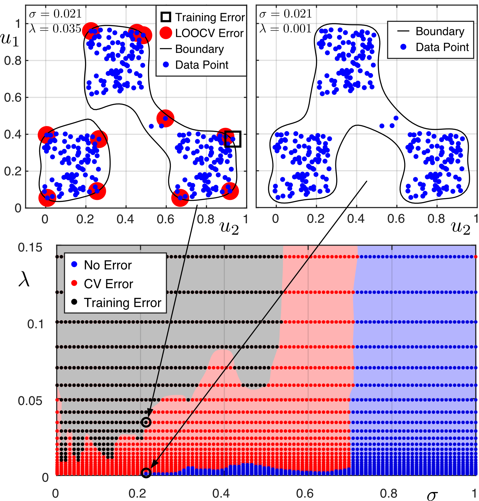
An example is given in Fig. 3. The bottom diagram indicates the hyperparameter areas that cause either training errors (and LOOCV errors), only LOOCV errors, or no errors.

Figure 3: Hyperparameters σ, λ chosen by the proposed method.

 

The top right diagram shows the classification using the hyperparameter combination selected with the presented strategy (highest leftmost parameter combination in the blue area). As an example, a classification with a combination of hyperparameters in the training error region (which also includes LOOCV errors) close to the LOOCV error region is shown in the top left diagram. Indeed, one point is misclassified and 11 points very close to the boundary would be misclassified if they weren't part of the training data.

A modified version of the procedure is proposed for two-class classification.

• The target classification value for all data points of one class is 1, the target value of the data points of the other class is -1.
• The classification boundary is zero.
• The training error and LOOCV error for all combinations of the hyperparameters is calculated.
• The hyperparameters with zero (or smallest) training error and zero (or smallest) LOOCV error are chosen.
• From these the ones with the largest σ are selected to ensure the smoothest boundary.
• From these the one with the largest λ is selected to ensure maximum numerical robustness.

The main difference here is, that the hyperparameters with the largest σ are chosen instead of the smallest. The choice of the largest possible σ is desirable since it leads to the smoothest and therefore most robust classification boundary. But this strategy is not feasible with one-class classification, since here a sufficiently large σ always ensures zero training and LOOCV error. But the boundary, in this case, is just driven far away from the data points. However, a tight boundary is desirable, so it becomes useless for classification.

 

Structural Health Monitoring (SHM) using Probability Density Estimation

Mechanical structures under permanent dynamical load can suffer from sudden catastrophic failure. Therefore, they must be checked regularly for possible damages and critical components may have to be renewed in regular intervals even without visible damages to ensure safety. This costly procedure can be improved by permanently monitoring the health of the structure using sensors and data processing.

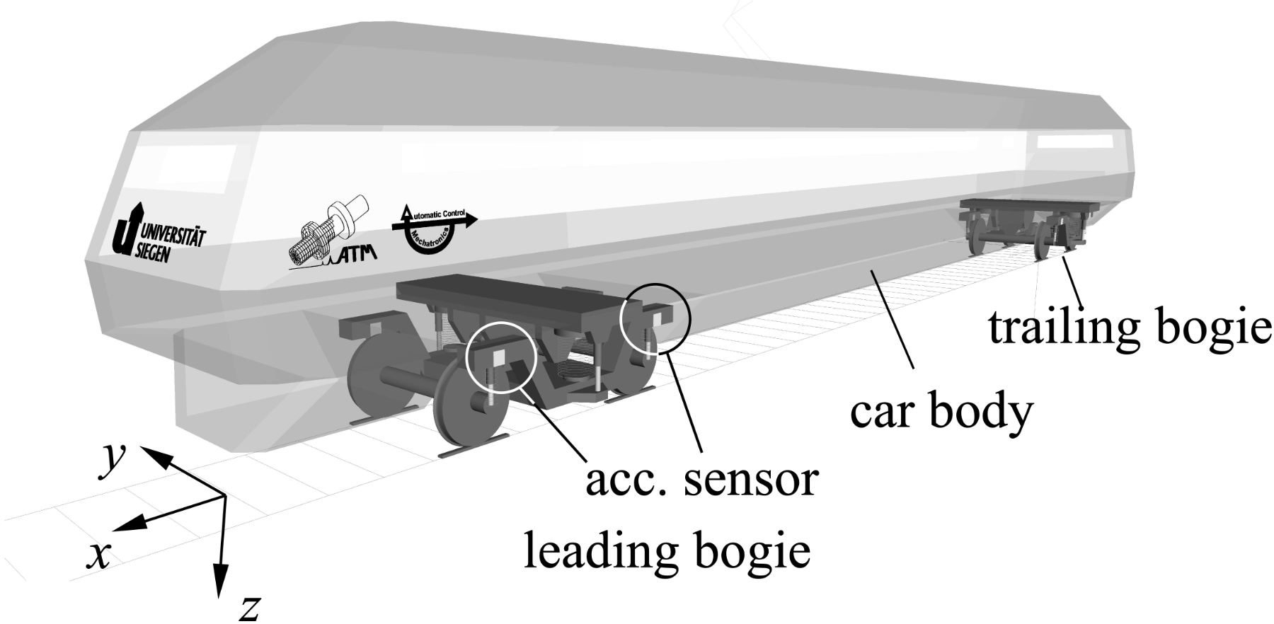
The operation of trains, for example, requires regular checks on the rail cars' bogies to avoid derailment e.g. caused by a defective suspension. Degradation of springs or dampers may be detected by mounting acceleration sensors on a bogie's frame and estimating the eigenfrequencies and modes of the mechanical system, see. Fig. 4.

Figure 4: Model of a train car with (simulated) acceleration sensors on the leading bogie.

 

The proposed structural health monitoring (SMH) system was tested in simulation using a (SIMPACK) multi-body model of a train car with two bogies and a simulated railtrack (ground and track model) [4]. The accelerations at two positions were calculated for a nominal suspension, and several cases where the suspension's springs were weakened by different degrees. Using an input-free subspace identification technique [4,5] (the input is assumed to be white noise) the eigenfrequencies and modes are estimated for short segments of the available data. In this way an SMH procedure is simulated that would operate online on a train.

For the subspace model used in the identification process a suitable model order must be assumed. One often used method, is to estimate the eigenfrequencies with an increasing model order until the eigenfrequencies stabilize at certain values. This procedure is usually aided by a stabilization plot where the estimated eigenfrequencies for each model order are plotted on top of each other.

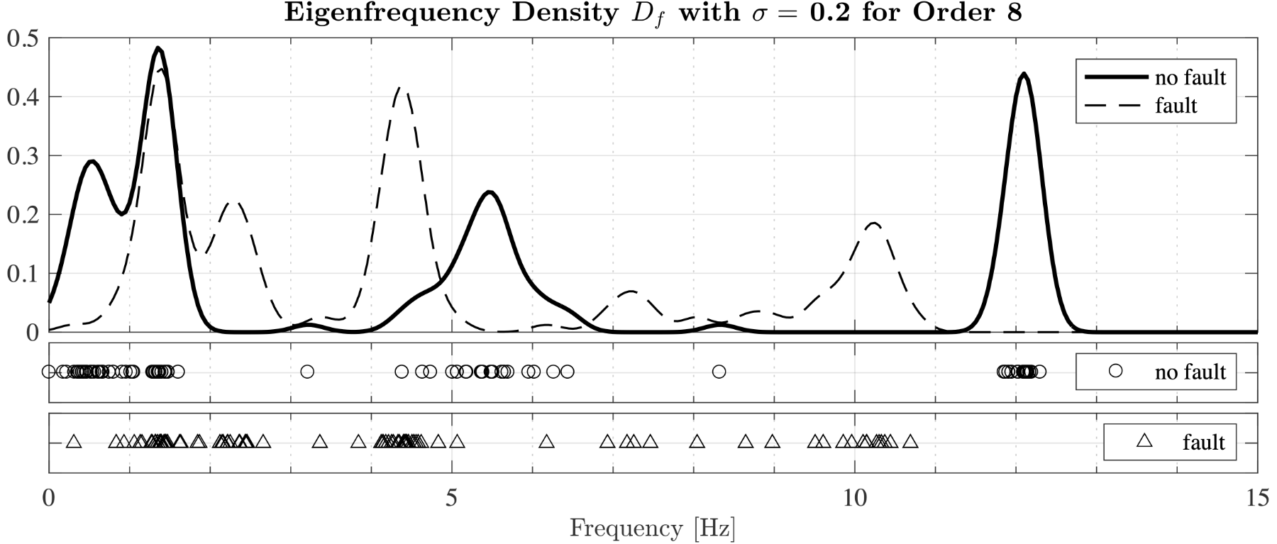
After collecting a suitable amount of fault-free (nominal suspension) data sets and estimating the eigenfrequencies for each set, it becomes clear that the results differ from dataset to dataset. This is caused by model error and changes in the excitation of the dynamic system caused e.g. by speed, curvature of the track, underground and so on. To mitigate this, it is proposed to estimate the eigenfrequency density [6] which shows how likely eigenfrequencies occur in certain value ranges. As an example, Fig. 5 shows eigenfrequency densities calculated from several data sets containing either a fault-free or faulty suspension. The fault-free eigenfrequencies are shown as circles in the plot and the corresponding density as a continuous line. The faulty eigenfrequencies are shown as triangles and the corresponding density as a dashed line.

Figure 5: Density of eigenfrequencies for fault-free and faulty cases.

 

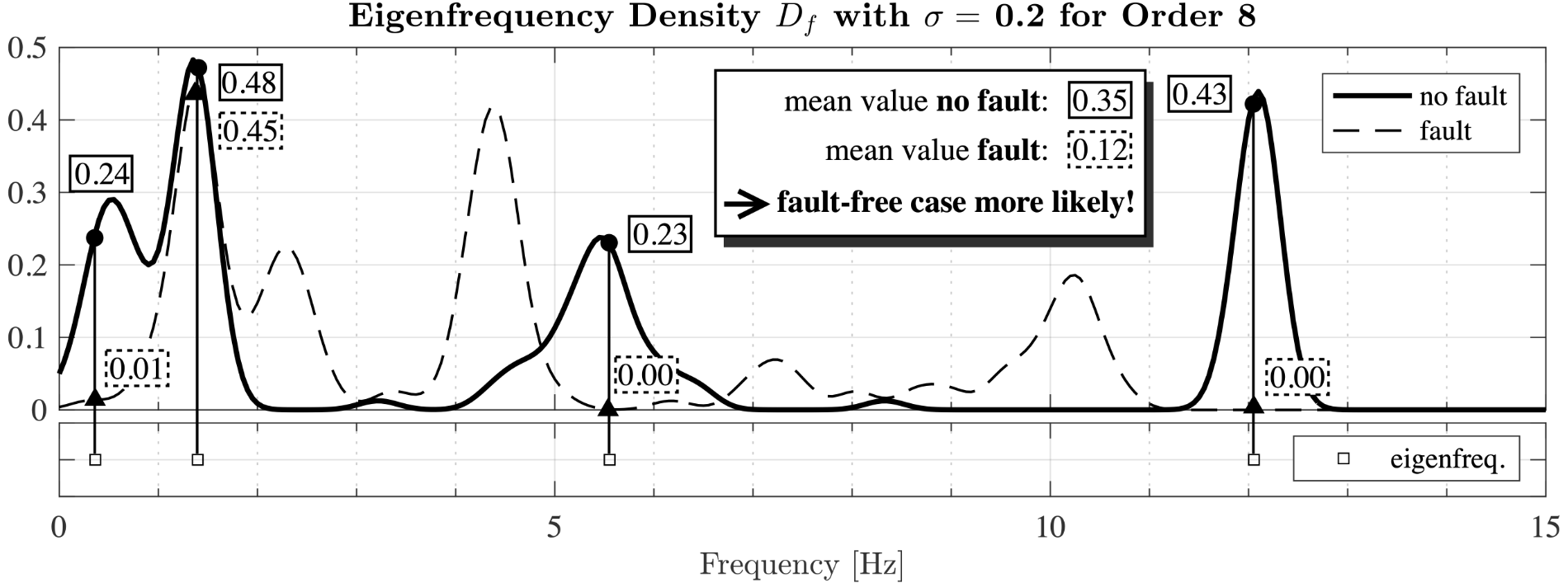
Even though the circle and triangles quite often overlap it can be seen at first glance that the densities for both cases strongly differ. This feature is used in the proposed SHM scheme to decide for new measurements if they indicate a fault-free or faulty suspension. This approach is depicted in Fig. 6. The squares at the bottom of the plot represent the four eigenfrequencies calculated from a newly acquired data set. At these four frequencies the values for both densities are determined and the average values are calculated respectively. It is now reasonable to assume that the new data set belongs to the case with the highest average density value, which, in this case, would mean that the suspension would be fault-free.

Figure 6: Determination, if a newly estimated set of eigenfrequencies corresponds to fault-free or faulty case.

 

The eigenfrequency density is calculated by placing one Gaussian on every eigenfrequency (the expected value equals the eigenfrequency) in the considered data set. Taking the mean value of all Gaussians achieves an overall probability of one. For this calculation the standard deviations of the Gaussians have to be chosen suitably. This can be done by minimizing the classification error using a cross-validation approach. The data sets are repeatedly randomly divided into two groups. One group is used for calculating the density (training data), the other one to calculate the classification error (validation data).

 

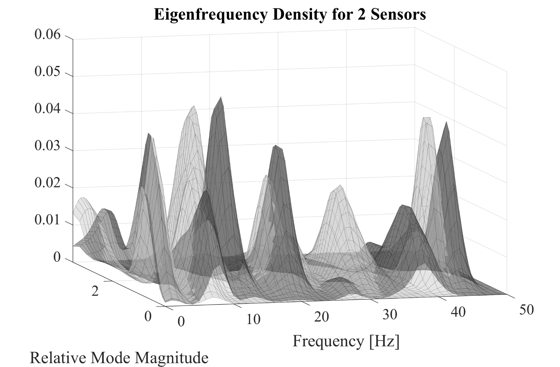
Figure 7: Using two sensors allows two-dimensional density over frequency and relative mode magnitude.

 

The SHM procedure described to far just needs one sensor. With additional sensors, beside the eigenfrequencies also the eigenmodes are available for fault detection. With one additional sensor two values for the mode can be calculated. As can be seen in Fig. 7, the relative mode magnitude (ratio of the two mode values) can now be used to calculate a two-dimensional density function. The two cases, fault-free (dark grey) and faulty (light gray), are visibly even better separated from each other than in the one-dimensional case, allowing for a more precise classification. Future research will investigate if using additional sensors will provide a method to reliably detect different kind of faults or fault locations.

 

References

[1]	David M. J. Tax. "One-class Classification". In: Thesis Technische Universiteit Delft, 2001
[2]	Geritt Kampmann, Oliver Nelles., "One-Class LS-SVM with Zero Leave-One-Out Error", In IEEE Symposium Series On Computational Intelligence, 2014
[3]	Volker Smits, Max Schüssler, Geritt Kampmann, Christoper Illg, Tim Decker, and Oliver Nelles. "Excitation Signal Design and Modeling Benchmark of NOx Emissions of a Diesel Engine", In: CCTA 2022 - IEEE Conference on Control Technology and Applications, 2022
[4]	Henning Jung, Tobias Münker, Geritt Kampmann, G, Kevin Rave, Claus-Peter Fritzen and Oliver Nelles. "A Novel Full Scale Roller Rig Test Bench for SHM Concepts of Railway Vehicles". In: e-Journal of Nondestructive Testing, 2016, 21
[5]	Peter Van Overschee and Bart De Moor. "Subspace Identification for Linear Systems". In: Kluwer Academic Press, 1996
[6]	Henning Jung, Tobias Münker, Geritt Kampmann, Oliver Nelles, and Claus-Peter Fritzen. "A probabilistic approach for fault detection of railway suspensions". In: International Workshop on Structural Health Monitoring, 2017

 

Next Topic

Previous Topic

Back to Overview