Research Topics Fabian Schneider
Data-driven Optimization of Multi-Stage Forming Processes
Modern development methods include more and more frequently model-based optimization strategies. Here, a model predicts the desired output of a process for given or selected process parameters, which are used as model inputs. Afterwards, a suitable optimization method is applied to find, based on the model, the process parameters which yield the optimal process results.
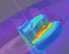
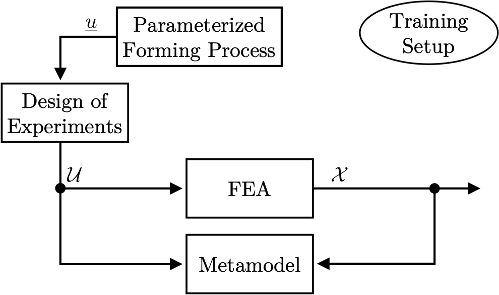
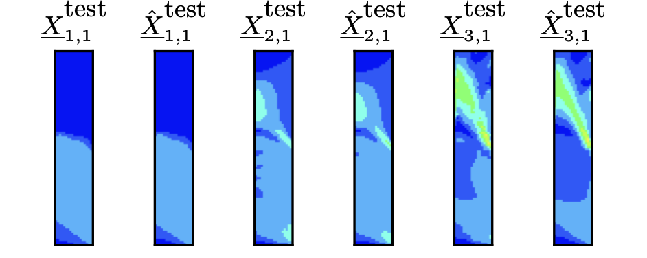
Such a data-driven optimization approach is applied to multi-stage forming processes. One particular quality measure is the equivalent plastic strain ϵpl. It describes the deformation of the raw material. Since it is impractical to measure ϵpl during a forming process, physics-based first principle models are used to calculate it, typically through a finite element analysis (FEA) an example is shown see Figure 1. Unfortunately, the FEA is not well suited for optimization processes. The computational costs of a simulation are too high. A data-driven model can significantly reduce computational costs compared to a physics-based model. Most data-driven models are computationally cheap and fast to evaluate. In this case, the data-driven model is a metamodel, a data-driven model of a first principle-based model (FEA). The typical training setup for a metamodel is shown in Figure 2. The model created should be able to predict the distributions of the process variables (e.g., ϵpl). This is important because the loss function can change during the development process. In addition, the spatial distribution also influences process quality. To make it possible to model such a spatial distribution of the process variables in 2D or even 3D, it is compressed into a two- to five-dimensional feature vector using an autoencoder. This feature vector can then be approximated using a second model. This can be carried out at different points in time for each simulation. In this way, predicting the distribution of the process variables over time is possible. Based on this overall model, process optimization can be done quickly and efficiently. An example for metamodel predictions is shown in Figure 3.
|
| Figure 1: Finite element analysis of a forming process. |
|
| Figure 2: Training setup of a metamodel. |
|
| Figure 3: Metamodel prediction of a multi-stage forming compared to the corresponding original data. |
Growing Design of Experiments with 1- and 2-Class Classifiers
Many industrial applications have a restricted parameter space. This means certain parameter combinations lead to destructive or undesirable process behavior and are, therefore, unfeasible. If a data-driven model of the process is to be generated, data must first be measured. At the same time, the exact process limits are often yet to be discovered. These can usually be estimated using process knowledge or simulations, but often not precisely enough. This is the case with combustion engines, for example. In practice, a two-step procedure is therefore used. First, the design limits are determined during an initial measurement phase. In an intermediate step, a measurement plan is then created considering these limits using a design of experiments. This measurement plan is finally executed in a second test bench run.
The method presented here combines both above descibed steps into a single one to reduce test bench time and cost. The parameter space is explored from a feasible (safe) initial point. To avoid excessive violations of the constraints, newly reached process points may only be located in the neighborhood of points that have already been visited.
Three primary requirements must be met for most applications:
- Space-filling desig
- Limited propagation speed
- Modeling of the constraint
Space-filling: To estimate high-quality data-driven models of hardly known processes with the smallest possible number of experiments, the valid parameter space must be covered completely and evenly. To achieve good coverage, each iteration selects the feasible point that leads to the best point distribution according to a space-filling criterion named ϕp .
Limited propagation speed: The transition to the unsustainable range of a process is often continuous rather than abrupt. A combustion engine, for example, runs unsteadily or begins to knock instead of failing immediately. This is why slight constraint violations are permitted during the measurement. A Robust One-Class Classifier (OCC) (Link) is used to ensure this. This OCC is trained for all feasible points in each iteration. Only a point close to the classification boundary is added in each iteration. The points for which this condition applies are called candidate points. From all candidate points the one, which optimizes the space filling criterion, is selected for the next measurement. The propagation speed can thus be regulated via the permitted distance to the (or all) previous measurement(s).
Modeling the constraint: A two-class classifier is used to model the constraint. This classifier can be trained as soon as one point becomes unfeasible. It is also updated in each iteration. As soon as the classifier is available, only points within the estimated feasible parameter space are tested. Thus, the accuracy of the model improves with the progress of the procedure.
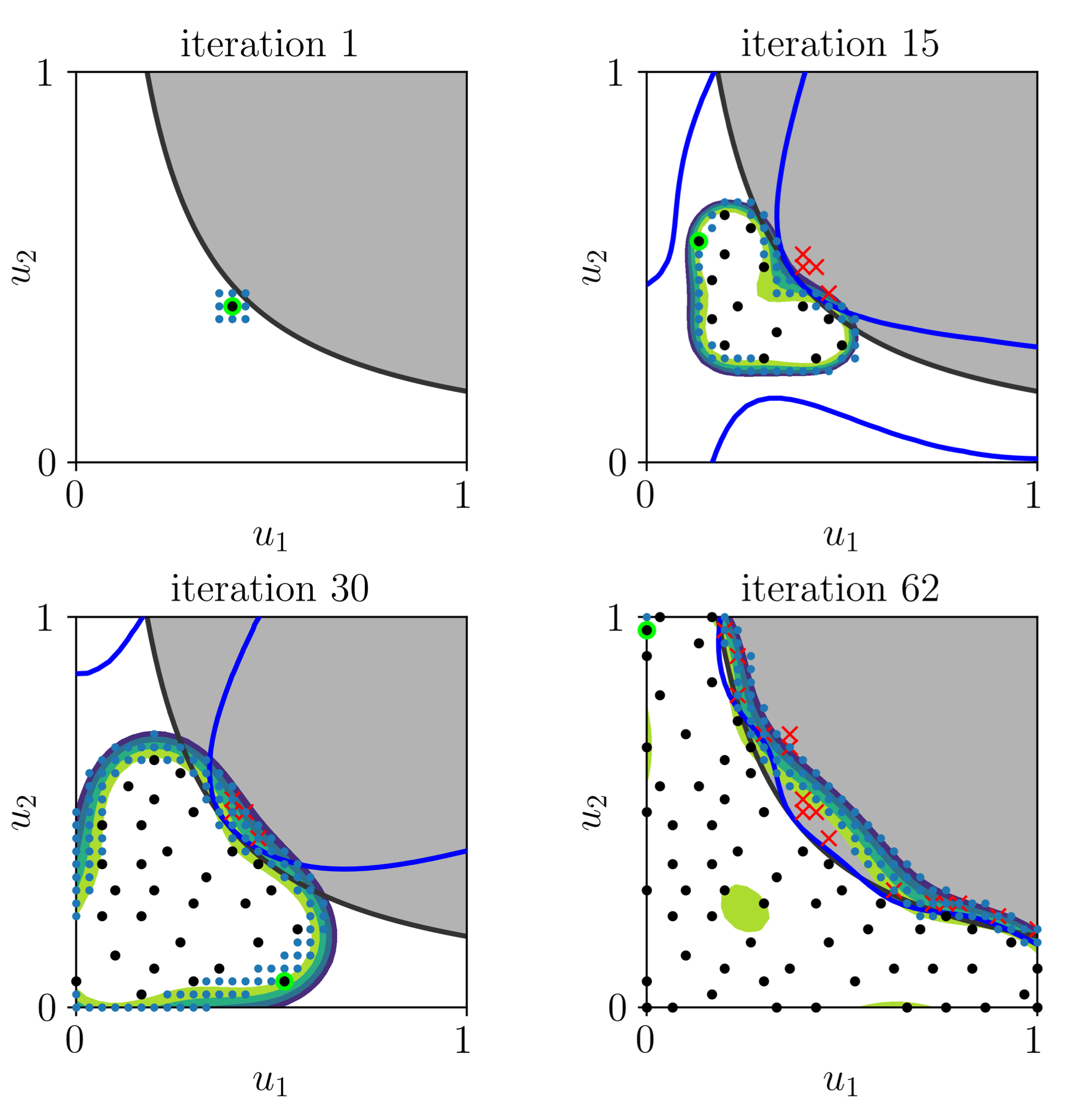
The procedure for a two-dimensional example process is shown below in Figure 4. The unfeasible parameter space is marked in gray. The boundary between feasible and unfeasible space is the black line. The black dots represent all points in the generated design. Red crosses mark tested points that are unfeasible. Blue dots are candidate points from which new points can be selected in each iteration. The contour band visualizes the one-class classifier. The blue line is the classification boundary of the two-class classifier.
Result: The constraint can be modeled without violating it too much. The entire feasible parameter space is evenly covered with measurement points.
|
| Figure 4: Example for 2-dimensional search for a feasable parameter space. |
LOLIMOT Lookup Tables
Lookup tables play an important role in static data-driven modeling. They are often applied to describe nonlinear processes, e.g. characteristics of combustion engines or automotive battery resistance estimation. In most cases they are grid-based, i.e., the supporting points lie on a regular grid. Each supporting point is associated with a height which is the output value at the corresponding input. Generalization between the supporting points is done by bilinear interpolation.
The popularity of lookup tables, however, results from the following combined design of experiments (DoE) & modeling strategy, which is trivial:
- Fix the granularity of all input variables, i.e., the number of levels for each axis.
- Establish supporting points at all level combinations (tensor product).
- Measure the process at all supporting points and set the heights equal to the measured outputs.
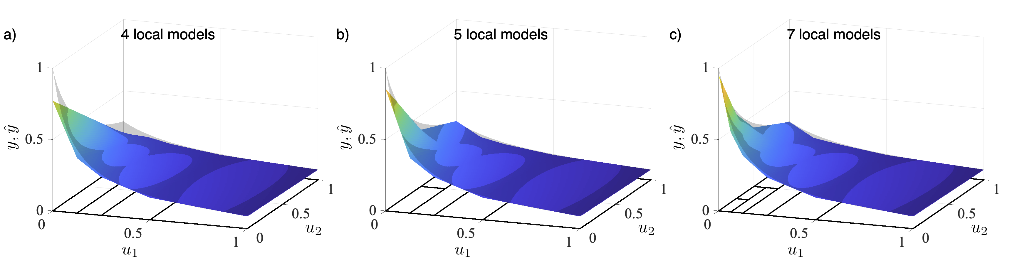
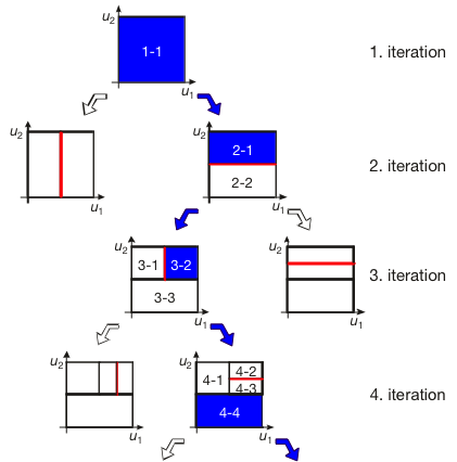
This strategy builds a model without any estimation/optimization step and is extremely simple. However, it enforces the use of a grid-based measurement strategy. It is also possible to measure data arbitrarily, not on a grid. Then the heights at all supportings points need to be estimated. If the supporting points have been fixed, this can be accomplished by least squares (LS). Grid-based approaches do not allow local refinement, so many unnecessary points must be measured. The number of unnecessary points rises strongly with increasing dimensionality. To make lookup tables much mor efficient for those cases, the grid-based approach is replaced by the local refinement strategy of the LOLIMOT construction algorithm, see Figures 5 and 6. Thus, model flexibility can be increased only in the necessary regions, and less data is required in all other regions. The construction algorithm defines the supporting points. So, the heights can be estimated with least squares and quadratic programming. It is also possible to measure the required support points directly. This results in an effective design of experiments strategy.
|
| Figure 5: Model approximation and partitioning for a) 4, b) 5, and c) 7 local bilinear models. |
|
| Figure 6: Local linear model tree (LOLIMOT) construction algorithm. |