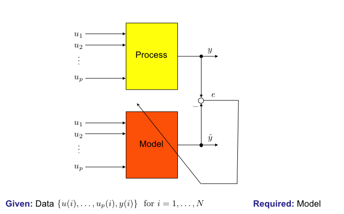
1. Experimental Modeling (Identification)
Vision: Automatic Modeling
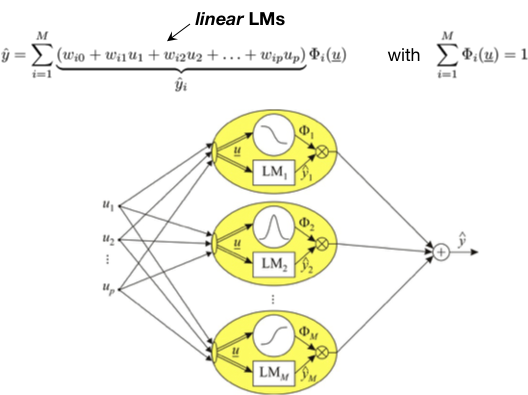
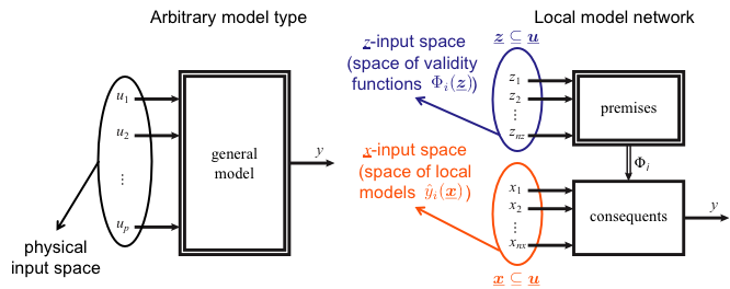
Local Model Network
Introduction
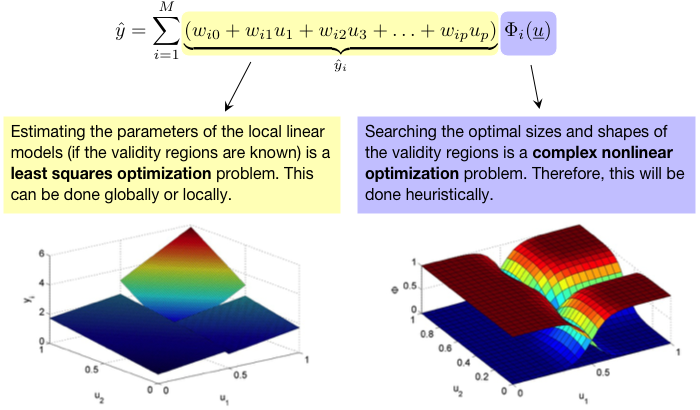
Model output is calculated by summing up the contributions of all M local models (LMs):
Advantages
- Separate input spaces for validity functions (rule premises) z and local models (rule consequents) x.
- Local estimation of local model parameters much more robust → Regularization.
- Local models can be of arbitrary type:
- linear: number of parameters scale linearly with dim(x)
- quadratic: optimization,
- higher order polynomials: subset selection or ridge regression required,
- from first principles: prior knowledge effectively utilized. - Exact shape of validity function not relevant.
- Efficient greedy learning strategies are available.
Drawbacks
- Undesired interpolation side effect.
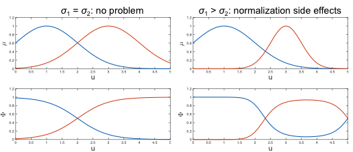
- Undesired normalization side effects.
- Suboptimal.
Separate Input Spaces for Validity Functions z and Local Models x
- Additional flexibility.
- Better interpretation.
- z can be seen as scheduling variables (often low-dimensional).
- x often is high-dimensional, particularly for dynamic systems.
Interpretation as Takagi-Sugeno Fuzzy System
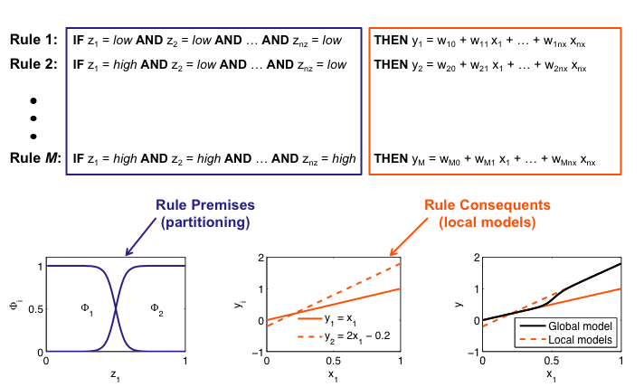
Partion of Unity
![]()
Two Ways to Achieve This
1. Normalization based on Gaussians: - Defuzzification
- Undesirable side effects
2. Hierarchy based on sigmoids
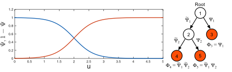
- Binary tree
- Knots weighted with Psi and 1-Psi
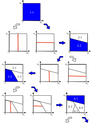
Algorithm 1: Local Linear Model Tree (LOLIMOT)
Properties:- Partitioning: Axes-orthogonal.
- Structure: Flat (parallel).
- Splitting functions: Normalized Gaussian functions.
- Splitting method: Heuristically, without nonlinear optimization.
LOLIMOT Construction Algorithm
- Incremental (growing) algorithm: Adds one LM in each iteration.
- Split of the locally worst LM.
- Test of all splitting dimensions and selection of the best alternative.
- Local least squares estimation of the LM parameters.
- Use normalized Gaussian validity functions.
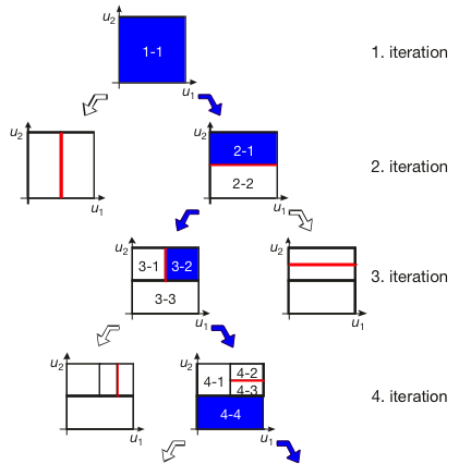
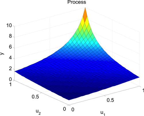
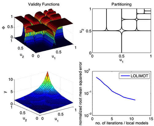
Demonstration Example (Hyperbola)
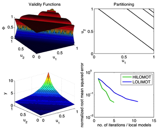
Algorithm 2: Hierarchical Local Model Tree (HILOMOT)
Properties:
- Partitioning: Axes-oblique.
- Structure: Hierarchical.
- Splitting functions: Sigmoid functions.
- Splitting method: Nonlinear optimization of sigmoid parameters.
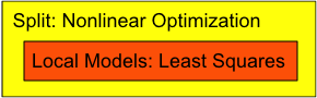
HILOMOT Optimization
- Nested approach.
- Separable nonlinear least squares.
- Outer loop: Gradient-based nonlinear optimization of split.
- Inner loop: One-shot least squares (LS) optimization of local model parameters.
Enhancements
- Regularization of LS optimization (ridge regression).
- Subset selection instead of LS can determine local structure.
- Constraint nonlinear optimization of the splits guarantees for all local models
 .
. - Analytical gradient calculation speeds up optimization by factor dim(u).
- Derivative of inverse matrix (LS estimation) necessary.
- Automatic sophisticated smoothness adjustment of sigmoid splitting functions.
Separable Nonlinear Least Squares
HILOMOT: Extension and Modification of LOLIMOT
- Incremental (growing) algorithm: Adds one LM in each iteration → like LOLIMOT.
- Split of the locally worst LM → like LOLIMOT.
- Optimize splitting position and angle by nonlinear optimization → new.
- Automatic smoothness adjustment algorithm → new.
- Local least squares estimation of the LM parameters → like LOLIMOT.
- Use sigmoid validity functions → different to LOLIMOT.
- Build up a hierarchical model structure → different to LOLIMOT.
Demonstration Example (Hyperbola)
Properties of LOLIMOT
- Axes-orthogonal splits.
- Flat structure can be computed in parallel.
- Strongly suboptimal in high dimensions.
- Faster training.
- Easier to understand and interpret.
- Normalization side effects.
Properties of HILOMOT
- Axes-oblique splits.
- Hierarchical structure fully decouples local models.
- Well suited for high dimensions.
- Analytical gradient calculation for split optimization.
- Superior model accuracy.
- No normalization numerator (defuzzification). → No reactivation effects. Hierarchy automatically guarantee a ‘partition of unity’.
- Sigmoids are easier to approximate than Gaussians for microcontroller implementation.
Summary: Advantages of Local Model Networks
- Incremental → all models from simple to complex are constructed.
- Local estimation:
- All local model are decoupled.
- Extremely fast.
- Regularization effect → almost no overfitting. - Local model are linear in their parameters:
- Global optimum is found.
- Robust & mature algorithms for least squares estimation are utilized.
- Structure selection technique can be applied.
- Adaptive models → recursive algorithms can be applied. - Local model can be of any linearly parameterized type: constant, linear, quadratic, ...
- Different input spaces for validity functions (rule premises) and local models (rule consequents) → new approaches to dimensionality reduction.
- Complex problem is divided into smaller sub-problems (local models) → divide & conquer.
- Many concepts from the linear world can be transferred to the nonlinear world → particularly important for dynamic models.
LMNtool
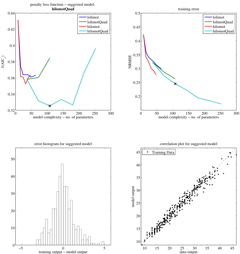
- MATLAB toolbox.
- Object-oriented programming.
- Local linear and quadratic models.
- LOLIMOT (axes-orthogonal partitions).
- HILOMOT (axes-oblique partitions).
- Model complexity chosen according to corrected Akaike information criterion.
- Analytical gradient calculation for high training speed
- Reproducible results
- All fiddle parameters can keep their default values. No expertise required.
- Trivial usage:
